Merkle Tree Construction and Proof-of-Inclusion

Trees are one of my favorite concepts. It's amazing how much of the real world can be mapped to trees and graphs. One interesting types of tree and the subject of this article is called a Merkle tree. Merkle trees are used in Bitcoin and provide a fascinating way to efficiently prove the existence of data. This article assumes you have a basic understanding of cryptographic hash functions as well as basic binary tree algorithms.

Basics

A Merkle tree is a type of hash tree that was invented by cryptographer Ralph Merkle. It is a binary tree, where a node can only have zero, one, or two children. This type of tree uses hashes for the leaves of the tree. Interior nodes are constructed by concatenating the hashes of the children and taking a hash of that result. The tree is complete when there is a single node, which is called the Merkle root. Below is an example of a four node Merkle tree.

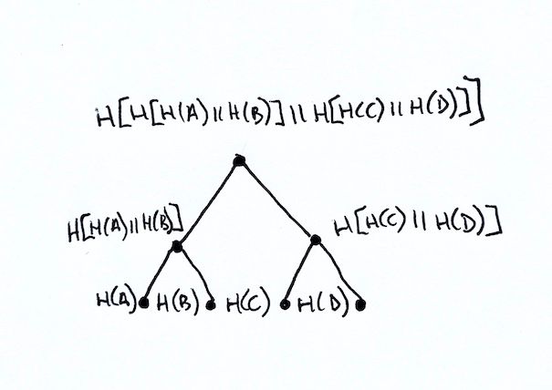
Starting from the bottom, you can see that the leaves consist of the hash via function H of values for the nodes a, b, c, and d.  The leaves are paired and the hash of those values is used to construct the value for the parent nodes
H[H(a)||H(b)] and  H[H(c)||H(d)].  Finally the root is constructed by hashing the two parent nodes: H[ H[H(a)||H(b)] || H[H(c)||H(d)] ].

For the rest of this article and for simplicity sake, we will imply that each step performs concatenation and hashing. As a result we can simply refer to a node by  the result of this hashing. For instance if A = H(a) and B = H(b) then
AB = H(A||B) = H[H(a)||H(b)].

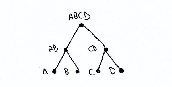
With this nomenclature, our four node example has the leaves A, B, C, and D.  The parents of the leaves are AB and CD.  Finally the root is ABCD.

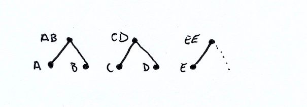
The above example is a best case scenario. The number of leaves is a power of two, which means we can pair things nicely all the way till we reach the root.  What happens if we have an odd number of leaves? What happens if an interior level has an odd number of nodes?  

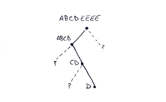
When constructing a Merkle tree, if we have an odd number of nodes at a particular level, we simply concatenate the last node with itself!  Consider a five node example with leaves A, B, C, D, and E.  

Here we have an odd number of nodes. So we will need to combine E with itself. We end of with pairs AB, CD, and EE.  

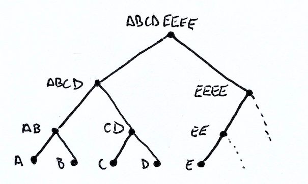
At this next level we again have an odd number of nodes: AB, CD, and EE.  So we again duplicate the last node and end up with ABCD and EEEE. Finally we join the last two nodes and end up with ABCDEEEE as our Merkle root!

Armed with this information, let's consider a construction algorithm.

Construction Algorithm

For me, it is easiest to conceptualize this tree using a pointer-based construction instead of an array-based construction. With pointers we can easily see that an interior node has either one child or two and we can use this knowledge to correctly compute the hash.

Because the information we are starting with is based on the leaves, we will also be constructing the tree from the leaves to the root using a bottom-up construction algorithm.

So let's start with the type, we call our type MerkleTree and it contains two children left and right that are both MerkleTree.  We also have hash property that stores the value of the current node.

export class MerkleTree {
    /**
     * Left subtree
     */
    public left: MerkleTree;

    /**
     * Right subtree
     */
    public right: MerkleTree;

    /**
     * Hash that is either provide or populated
     */
    public hash: Buffer;

    /**
     * Computes the hash based on the children. If no right child
     * exists, reuse the left child's value
     */
    public computeHash(): Buffer {
        const leftHash = this.left.hash;
        const rightHash = this.right ? this.right.hash : leftHash;
        return hash256(Buffer.concat([leftHash, rightHash]));
    } 
}

This class also has a computeHash function that detects whether the node has a single child and will duplicate the left node automatically in the hash calculation. The function uses a hash256 hash algorithm, which is commonly used in Bitcoin and consists of a double-SHA256 hash, SHA256(SHA256(value)).

Now that we have a basic structure we will create our fromHashes method that will construct a Merkle tree from a list of hash values.

function fromHashes(hashes: Buffer[]): MerkleTree {
    // Convert the initial hashes into leaf nodes. We will use these 
    // leaf nodes to construuct the Merkle tree from the bottom up by 
    // successively combining pairing nodes at each level to construct 
    // the parent
    let nodes = hashes.map(p => new MerkleTree(p));

    // Loop until we reach a single node, which will be our Merkle root
    while (nodes.length > 1) {
        const parents = [];

        // Successively pair up nodes at each level 
        for (let i = 0; i < nodes.length; i += 2) {
            // Create the parent node, which we will add a left, try add 
            // a right, then calculate the hash for the node
            const parent = new MerkleTree();
            parents.push(parent);

            // Assign the left, which will always be there
            parent.left = nodes[i];

            // Assign the right, which won't always be there. However,
            // in JavaScript, an array overflow simply returns undefined
            // which in this context, is the same as a null pointer.
            parent.right = nodes[i + 1];

            // Finally compute the hash, which will be based on the 
            // number of children.
            parent.hash = parent.compuuteHash();
        }

        // Once all pairs have been made, the parents now become the 
        // children and we start all over again
        nodes = parents;
    }

    // Return the single node as our root
    return nodes[0];
}

This algorithm isn't too complicated. The first thing we do is convert the hashes into child nodes. Then we initiate our construction loop until we only have a single node, which will be our Merkle root.

For each level of construction we pair the nodes and construct a new node as the parent. We use our computeHash function to calculate the new node's hash. When all the pairs are processed, we make these new pairs the subject of the next round of processing! When all is said and done, we should be left with a single node that is our Merkle root.

With a construction algorithm, you can now compute the root from a list of hashes. This is useful for seeing if any of the leaves have changed. For instance, you could use this to validate that a catalog of files has not changed. If any of the files change, it would would change the root and all of that file's parent node's hashes.

You could also use this algorithm to validate a Bitcoin block. You could take the leaves as the transaction identifiers and calculate the Merkle root that is included in the block header. One caveat with Bitcoin Merkle trees is that block explorers and public facing transaction identifiers use a reversed byte order. The Bitcoin Merkle tree is constructed using the internal byte ordering (or natural ordering) of the transaction identifiers not the public or RPC byte order.

One other interesting use case is called a "proof-of-inclusion".  This type of proof allows us to provide some information about the path through the Merkle tree that to proves a leaf is in the tree.

Proof-of-Inclusion

A proof-of-inclusion for Merkle trees are very efficient for proving the existance of data. We do not need to reveal or calculate all of the information in the tree, only relevant pieces of information needed to traverse from the root to the desired leaf.

For trees we can reach a leaf in O(height). The height of the tree depends on the structure of the tree. Balanced trees mean that the leaves of the tree differ by no more than one level. Unbalanced trees can are abitrary in height and can range from log n to n-1 depending on the structure.  Fortunately, Merkle trees, are a balanced tree since the depth of the leaves always at the same height.  This means we can reach a node in O(log n) time complexity, which is incredibly efficient.

For example, a graph with 1 million nodes in it will only require 20 steps to reach the leaf from the root!  In comparison, if we were to use something like a hashchain where we simply concatenate and hash each leaf value successively we would need to provide all 1MM hashes as well as perform 1MM hash operations to prove our item is in the final result.

So let's consider what we are trying to accomplish: we know the root and we know the leaf. We want to provide a path that gets us from the root to the leaf.  As with most things with trees, we can start with a simple example and build off of it.

Given a tree with two leaves A and B, we end up with a Merkle root of AB.  

The pieces of information we know are the root AB, and a leaf  A. If we think about our construction algorithm, we already know A and we know we need to combine something with A. We also know the end result is going to be AB. So we need something to combine with A to get AB. Providing B allows us to calculate AB successfully, proving that we can recompute the root and that we A is required to compute that root!

If this seems obvious remember that hash functions are one way. That is given A and AB, there is no way to derive B.

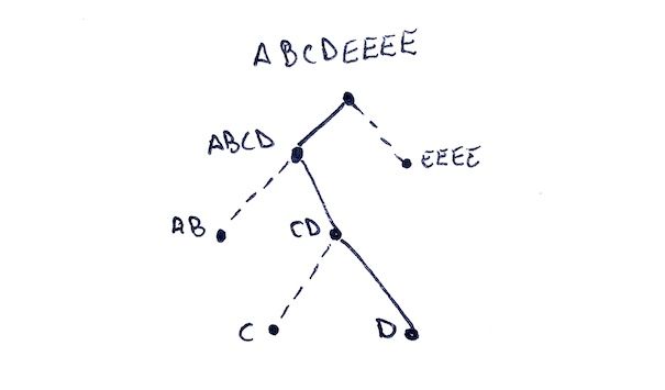
Let's create a slightly larger example to solidify what is going on here.  Let's take the tree with five nodes A, B, C, D, and E.  We know our root will be ABCDEEEE.  Our fully constructed Merkle tree is the same as before.

If we want to prove that D is in the tree, how do we go about this? Well think about what the missing pieces are along the path and what information is required to compute a parent's hash.

If we start at D and work our way upwards we would need to know its left sibling C.  This is needed to construct the parent hash CD.  With CD we would need to know its left sibling as well: AB. With AB and CD we can compute the hash ABCD. Finally with ABCD we would need its right sibling EEEE in order to calculate the root ABCDEEEE.  With all of those pieces we constructed a path from the root ABCDEEEE to the leaf.  

Flipping things around so we go from the root to the leaf is actually a bit easier to come up with an algorithm. When we visit a node it is going to be one of three types:

1. A leaf node that is our target
2. A node in our path
3. A sibling to a node in our path

If we look back at what we just constructed we can see that:

• ABCDEEEE is obviously in our path since its the root
• ABCD is in our path
• EEEE is a sibling of ABCD
• AB is a sibling of CD
• CD is in our path
• C is a sibling of D
• D is a leaf and is our target

Given this knowledge we can construct a path using a top-down traversal of the tree. We do this by building a collection of hashes of interest and using a bitfield to create a map of actions required to traverse the tree.

• If the node is in the path and is a leaf
     1. Push a 1 bit onto the bitfield
     2. Add the hash onto the list of hashes
• If the node is in the path
     1. Push a 1 bit onto the bitfield
     2. Calculate the hash after traversing left and then right
• Otherwise
     1. Push a 0 bit onto the bitfield
     2. Add the hash onto the list of hashes

If we apply this algorithm to our example above we have the following steps:

1. Starting at the root ABCDEEEE, the root is in the path, so we push a 1 and then traverse to left. After this step our values are:
      Bits: [1]
      Hashes: []
2. We are now at ABCD, this is also in our path, so we push another 1 and traverse left again. After this step our values are:
      Bits: [1,1]
      Hashes: []
3. We are now at AB, which is not in our path, so we push a 0 and add AB to our list of hashes. We immediately return to the parent. After this step our values are:
      Bits: [1,1,0]
      Hashes: [AB]
4. We are now back at ABCD and must finish the traversal by going right.
5. We are now at CD, which is in our path, so we push a 1 and traverse left. After this step our values are:
      Bits: [1,1,0,1]
      Hashes: [AB]
6. We are now C, which is not in our path. We push a 0 bit and push the hash for C. We immediately return to the parent. After this step our values are:
      Bits: [1,1,0,1,0]
      Hashes: [AB, C]
7. We are now back at CD and need to finish the traversal by moving right.
8. We are now at D, which in our path and is a leaf node. It also happens to be our target! We push a 1 bit and push the hash. We to the parent. The values after this step are:
      Bits: [1,1,0,1,0,1]
      Hashes: [AB, C, D]
9. We are now back at CD and have traversed left and right so we are done and return to the parent.
10. We are now back at ABCD and have traversed left and right so we are done and return to the parent.
11. We are now back at ABCDEEEE and have completed our left traversal but still need to traverse right.
12. We are now at EEEE which is not in our path. We push a 0 bit and the hash. We immediately return the parent. The values after this step are:
       Bits: [1,1,0,1,0,1]
       Hashes: [AB, C, D, EEEE]
13. We are now back at ABCDEEEE and have traversed left and right. We have completed the traversal!

The final values and the proof for a 5-node Merkle tree are:
   Bits: [1,1,0,1,0,1]
   Hashes: [AB, C, D, EEEE]

So our Merkle proof-of-inclusion must consist of the following pieces of information:

• Merkle root
• Number of nodes in the tree
• List of hashes
• List of bits

The number of nodes in the tree gives us the shape of the Merkle tree, which will always be the same given the number of nodes. Knowing the number of nodes allows us to calculate if we are visiting a leaf node or an interior node.

Validating a Proof-of-Inclusion

Given the Merkle root, number of nodes, list of hashes and list of bits allows us to reconstruct a partial Merkle tree. If we are able to reconstruct the partial Merkle tree successfully and the root matches the expected root, then we have verified the proof!

The algorithm for construction of a partial Merkle tree is similar to the algorithm used to build the partial tree.  We again use a top-down algorithm to read the bitfield and hashes:

• If the bit is 0, construct a node using the next hash and return.
• If the bit is 1 and is at leaf depth, construct a node using the next hash and return.
• If the bit is 1 and not at leaf depth, traverse left, then traverse right, then compute the hash and return.

We prove that our leaf is in the Merkle tree if we end with the expected Merkle root and we do not have any bits or hashes left when processing.

Armed with this knowledge, we can now write a function that takes the input data and reconstructs our partial Merkle tree. This reconstruction, if done without error will guarantee that our leaf node was part of the tree used to construct the root. Our function will return the root of the constructed tree.

function fromProof(total: bigint, bits: bigint, hashes: Buffer[]): MerkleTree {
    // create copy of hashes so we can shift values from the front 
    // without impacting the original list
    hashes = hashes.slice();

    // calculate the max depth of the tree which is ceil(log2(h))
    const leafDepth = Math.ceil(Math.log2(Number(total)));

    // Call the closure-scoped construction function that starts at 
    // depth of 0 and eventually returns the root. This function is 
    // defined below and mutates the hashes and total value along the way
    const root = construct(0);

    // Verify that everything was consumed
    if (bits > 0n || hashes.length) {
      throw new Error("construction failed");
    }

    // Finally return the root so you can compare it to the expected
    // root and verify the constructed path.
    return root;

    // Closure scoped function that performs a pre-order construction of 
    // the merkle tree. Pre-order means we traverse the tree in order: 
    // root, left, right. In this instance, we read the bit field of the 
    // parent before the children.
    function construct(depth: number) {
        // read and remove the least-significant bit which will provide 
        // meaning to the hashes that were provided
        const bit = bits & 1n;
        bits = bits >> 1n;
  
        // We will populate this value depending on what action 
        // needs to be taken give the current bit and depth
        let node: MerkleTree;
  
        // Leaf node always shifts off a hash value becuase it will 
        // either be a target (bit=1) and include a hash or it will be 
        // included hash (bit=0). Either way, there is no need to 
        // traverse further. Return undefined if no hashes remain, 
        // which can happen with an odd number of leaves
        if (depth === leafDepth) {
            const hash = hashes.shift();
            if (hash) node = new MerkleTree(hash);
        }
  
        // When bit=1, we are responsible for calculating the hash. 
        // We need to continue the traversal (left, then right) 
        // and can compute the hash once the traversal is complete.
        // Note that we recursively call construct and increase the 
        // depth as we move down the tree
        else if (bit === 1n) {
            node = new MerkleTree();
            node.left = construct(depth + 1);
            node.right = construct(depth + 1);
            node.setHash();
        }
  
        // When bit=0, we are given the hash value since it is a 
        // sibling to a node in our path. Return undefined if no hashes 
        // remain which occurs when there are an odd number of nodes 
        // at this depth
        else {
          const hash = hashes.shift();
          if (hash) node = new MerkleTree(hash);         
        }
  
        // Finally return the node or undefined depending on how things
        // played out
        return node;
      }
  }

This function uses a bigint value for the bitfield which enables us to have more than 31 bits of data and use bit wise operations. When this function executes it will eventually return a MerkleTree instance that is the root.

This function creates a closure-scoped internal helper to perform a pre-order traversal of the tree. We start at a depth of 0 and we remove the least-significant bit from the bitfield.

Using each bit, we determine what additional construction logic is required. The logic is going to be one of our three conditions we discussed previously.  

The most complex scenario is when it is an internal node (bit=1 and not at leaf depath). This requires us to traverse left and then right before calculating the hash. We recursively call our construct method and increase the depth by 1.  This allows us to full traverse the tree to the left before we process to the right.

Conclusion

Hopefully this article helped highlight how Merkle trees can be constructed and how you can use them to perform a proof-of-inclusion. If you would like to see a working example of similar code, you can check out my TypeScript port of an SPV node from Programming Bitcoin.

If you want a deeper dive, you can read BIP0037 which adds Bloom Filter support to Bitcoin and creates the merkleblock message for use in SPV nodes.